

By Benjamin Louis | 21 May 2020 |

Context
Writing R Markdown document makes possible to insert R code and its results in a report with a choosen output format (HTML, PDF, Word). It is a real asset for analysis reproducibility as well as communication of methods and results. Doing daily data analysis, I usually deliver outputs in report and R Markdown naturally became an essential tool of my workflow.
Data analysis without data visualisation is like playing darts in the dark, there is a good chance you’ll miss the bullseye point. You’ll find quite a few R packages to build graphics but I have a preference for ggplot2 (I’m not alone!). Therefore, ggplot2 graphics are often included in my R Markdown documents.
Features of both packages are highly flexible and you CAN always get what you want ! But if you are just starting out, getting what you want can be cumbersome. In this post, I share with you some tips found over time.
Requirements
- I assume you have already made a graphic with
ggplot2or at least seen someggplot2code. If not, you can have a look at this book freely available online. To avoid iris data, I will use a data visualisation of Palmer penguins data recently included in a R package by Allison Horst (go see her illustrations too !). I start with this graphic :
library(ggplot2)
p <- ggplot(penguins_raw, aes(x = culmen_length_mm, y = culmen_depth_mm, color = species, fill = species)) +
  geom_point() +
  geom_smooth(method = "lm", formula = "y ~ x", alpha = 0.3) +
  scale_color_viridis_d() +
  scale_fill_viridis_d() +
  labs(x = "Culmen Length (mm)", y = "Culmen depth (mm)", fill = "Species", color = "Species")
p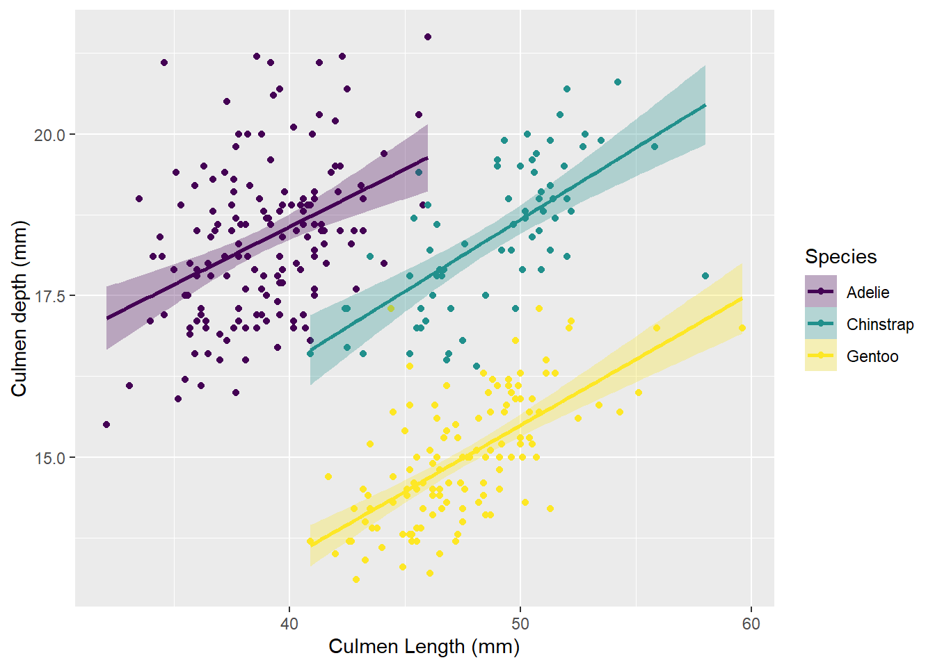
- Besides, it’s better if you know how to create a R Markdown document and you know how to include R code in it (with a chunk). If not, start here.
Making your own ggplot2 theme
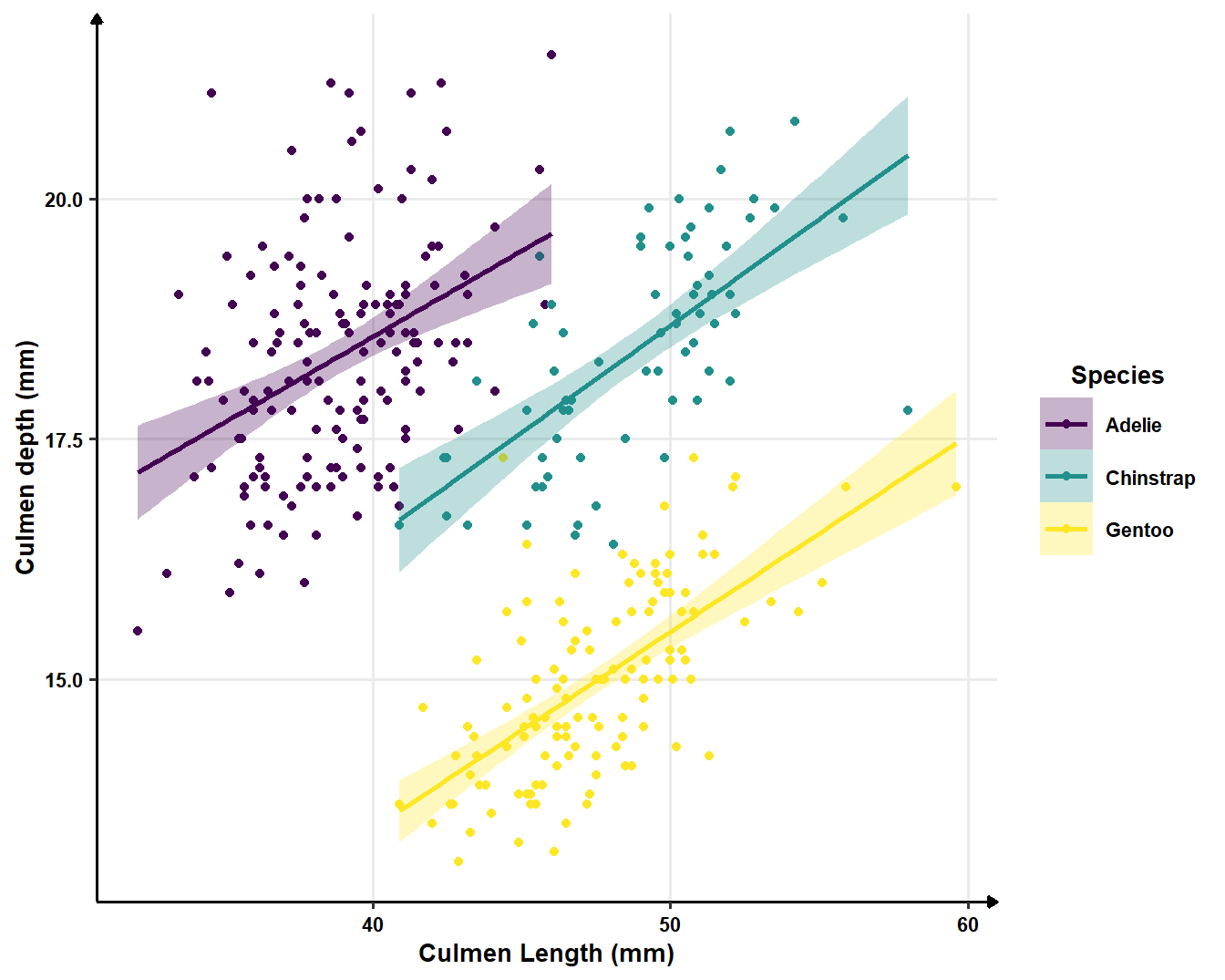
ggplot2 theme manages how your graphic looks like. All elemements can be changed through the theme() function but there also are pre-configured. The default theme used by ggplot2 is theme_gray() but I often switch for theme_bw() (for black and white).
p + labs(title = "Thème par défaut")
p + theme_bw() + labs(title = "Avec theme_bw()")
If you always use the same modifications with theme() function, I highly suggest that you create your own theme. Here is a customised one :
theme_ben <- function(base_size = 14) {
theme_bw(base_size = base_size) %+replace%
theme(
# L'ensemble de la figure
plot.title = element_text(size = rel(1), face = "bold", margin = margin(0,0,5,0), hjust = 0),
# Zone où se situe le graphique
panel.grid.minor = element_blank(),
panel.border = element_blank(),
# Les axes
axis.title = element_text(size = rel(0.85), face = "bold"),
axis.text = element_text(size = rel(0.70), face = "bold"),
axis.line = element_line(color = "black", arrow = arrow(length = unit(0.3, "lines"), type = "closed")),
# La légende
legend.title = element_text(size = rel(0.85), face = "bold"),
legend.text = element_text(size = rel(0.70), face = "bold"),
legend.key = element_rect(fill = "transparent", colour = NA),
legend.key.size = unit(1.5, "lines"),
legend.background = element_rect(fill = "transparent", colour = NA),
# Les étiquettes dans le cas d'un facetting
strip.background = element_rect(fill = "#17252D", color = "#17252D"),
strip.text = element_text(size = rel(0.85), face = "bold", color = "white", margin = margin(5,0,5,0))
)
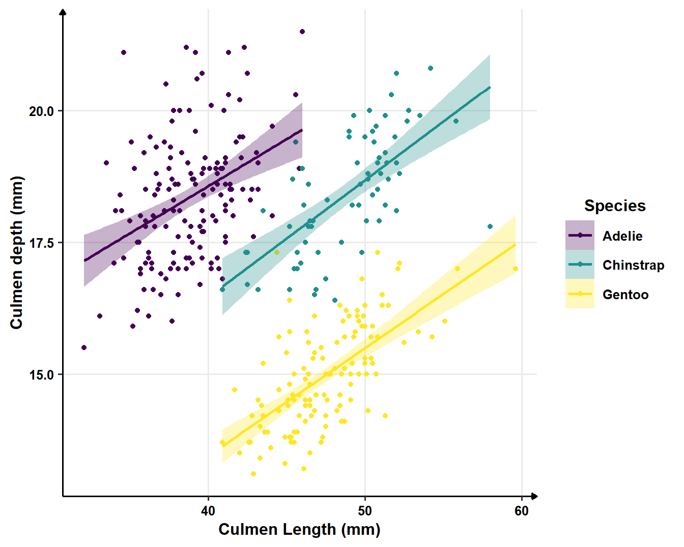
}And the results compared to the default one :
p + labs(title = "Thème par défaut")
p + theme_ben() + labs(title = "Avec mon thème personnalisé")
Building a customised theme is done by creating a R function where a pre-configured theme is used but some elements are modified with the theme() function. The tip is in the use of %+replace% in place of the classic +. unlike the latter, %+replace% doesn’t only update elements of a theme but replaces them entirely.
Now you just have to let your creativity flows. There are lots of editable elements so the customisation is pretty much limitless. You can find the list of elements in the webpage of the theme() function. In the example, the modified elements are for the whole figure (plot.* elements), the grapihic area (pnael.*), the axis (axis.*), the legend (legend.*) and the graphics labels (strip.*) when facetting is used.
In my opinion, axis and legends are essential elements so my choices go towards highlighted them through their relative size using rel() function which return a proportion a the base size (base_size) and bolding theme (face = "bold").
Customisation of a ggplot2 theme can first be hard work but if you are going to often use the same configurations, it’s worth it. There are plenty ressources on the web.You can also contact me, I’ll be glad to help.
You can now insert your theme in a chunk at the beginning of your R Markdown document to use it all along. You can also create a R package with your theme, among others, and load this package.
Your ggplot figure in R Markdown
Chunk options for figures
Inserting R cade and its results in a R Markdown document is possible through utilisation of a chunk which can take several options.
```{r option1 = valeur_option1, option2 = valeur_option2}
# Le code R ici
```
Some of these options are specifics to figures made with R :
Options linked to the size of these figures when produced by R
Options linked to the size of these figures in the final document
Size options of figures produced by R
Options fig.width and fig.height enable to set width and height of R produced figures. The default value is set to 7 (inches). When I play with these options, I prefer using only one of them (fig.width) in association with another one, fig.asp, which sets the height-to-width ratio of the figure. It’s easier in my mind to play with this ratio than to give a width and a height separatetly. The default value of fig.asp is NULL but I often set it to \(0.8\), which often corresponds to the expected result.
Size options of figures produced by R have consequences on relative sizes of elements in this figures. For a ggplot2 figure, these elements will remain to the size defined in the used theme, whatever the chosen size of the figure. Therefore a huge size can lead to a very small text and vice versa.
fig.width = 3 - figure elements too big
```{r fig.asp = 0.8, fig.width = 3}
p + theme_ben()
```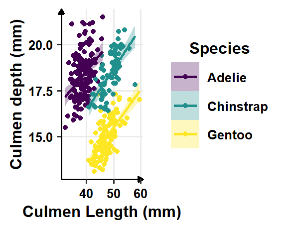
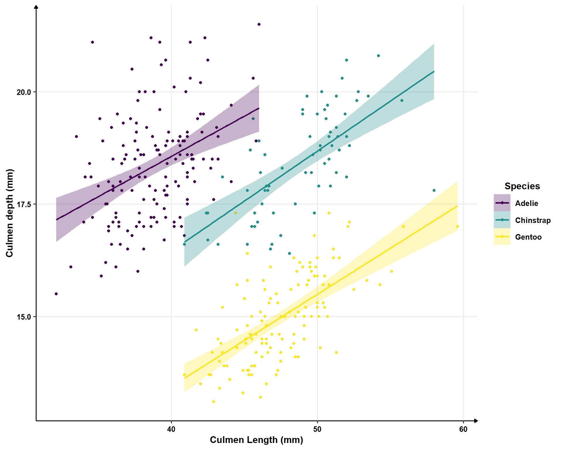
fig.width = 10 - figure elements too small
```{r fig.asp = 0.8, fig.width = 10}
p + theme_ben()
```
To find the result you like, you’ll need to combine sizes set in your theme and set in the chunk options. With my customised theme, the default size (7) looks good to me.
```{r fig.asp = 0.8, fig.width = 7}
p + theme_ben()
```
When texts axis are longer or when figures is overloaded, you can choose bigger size (8 or 9) to relatively reduce the figure elements. it’s worth noting that for the text sizes, you can also modify the base size in your theme to obtain similar figures.
fig.width = 9 - base_size = 14 (default)
```{r fig.asp = 0.8, fig.width = 9}
p + theme_ben(base_size = 14)
```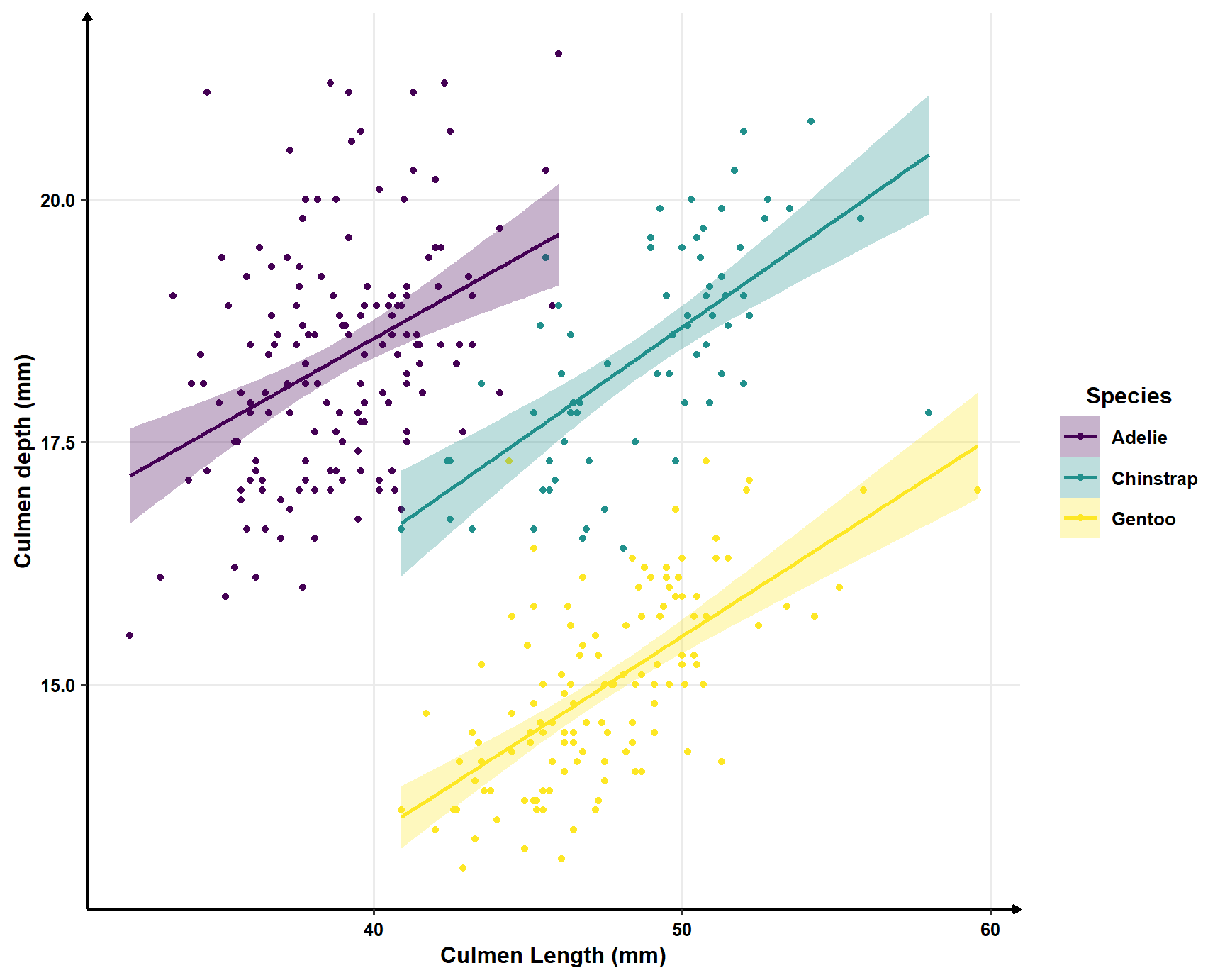
fig.width = 7 (default) - base_size = 12
```{r fig.asp = 0.8, fig.width = 7}
p + theme_ben(base_size = 12)
```
Size of figures in the final document
Figures made with R in a R Markdown document are exported (by default inpng format) and then inserted in the final rendered document. Options out.width and out.height enable to choose the size of the figure in the final document.
it is rare I need to rescale height-to-width ratio after the figures were produced with R and this ratio is kept if you modify only one option therefore I only use out.width. i like to use percentage to define the size of output figures. For example with a size set to 100% :
```{r fig.asp = 0.8, fig.width = 7, out.width = "100%}
p + theme_ben()
```
and a size set to 50% :
```{r fig.asp = 0.8, fig.width = 7, out.width = "50%}
p + theme_ben()
```
You can see here that the relative size of elements in the figure are unchanged. The figure is just more or less big.
Don’t repeat yourself
it’s kind of annoying to write several time the exact same thing. Here, for every chunk with a ggplot2 figure, you need to tell that you want it with your newly customised theme and you have to configure chunk options each time. Don’t worry, solutions to deal with your (my!) lazyness exist.
Changing default ggplot2 theme
You can change the default ggplot2 theme with the theme_set() function. You just have to write this line after creating your own theme (or loading the package with the theme you want) :
:
theme_set(theme_ben()) # change theme_ben() with the wanted themeChanging default values of chunk options
You can also change default values of chunk options by writing this at the beginning of your R Markdown document :
```{r setup, include=FALSE}
knitr::opts_chunk$set(
 fig.width = 6,
 fig.asp = 0.8,
 out.width = "80%"
)
```
These values will be applied for all chunks unless you specify other value in a chunk locally. You can set values often used (which differ from the default one) and avoid repeating them for each chunk.
What can be the beginning of your R Markdown document
With all these tips, here I show an example of the beginning of a R Markdown document (HTML output format) with customised theme and chunk options :
---
title: "My awesome title"
author: "Benjamin Louis"
date: "25/06/2020"
output: html_document
---


```{r setup, include=FALSE}
# Chunk options
knitr::opts_chunk$set(
 fig.width = 6,
 fig.asp = 0.8,
 out.width = "80%"
)
```

```{r theme_ggplot2, echo = FALSE}
# Creating a ggplot2 theme
library(ggplot)
theme_ben <- function(base_size = 14) {
  theme_bw(base_size = base_size) %+replace%
    theme(
      # changed theme options
    )
}
# Changing the default theme
theme_set(theme_ben())
```
From now on, you can modify what you need to create your ggplot2 theme et give chunk options you like better. Of course, these options are not limited to figures produced by R, you can look at this webpage to discover others.
I hope this post will help you write report you like and feel free to share your tips in the comments section !
Data citations
Palmer penguins data where originally published in : Gorman KB, Williams TD, Fraser WR (2014) Ecological Sexual Dimorphism and > Environmental Variability within a Community of Antarctic Penguins (Genus Pygoscelis). PLoS ONE 9(3): e90081. > doi:10.1371/journal.pone.0090081